Predicting the Premier League with Dixon-Coles and xG

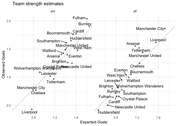
Recently, I ran through Predicting the Premier League with Dixon-Coles. I was interested in seeing how these predictions change when we use xG, rather than observed goals. So I’ve run some quick comparisons using xG data from understat.com.

The method will be largely the same as the previous post, so I’m going to keep comments on the code relatively light. If anything remains unclear, I’d suggest running through the code yourself (it should be reproducible on your computer - let me know if it’s not), or referring to the previous post.

Fetch the data

I’ll be using from understat (pasted onto GitHub), which you can access via the shortlink below:

library(tidyverse)
library(regista)

data <-
read_csv("https://git.io/fhsnd") %>%
nest(side, xg, .key = "shots") %>%
factor_teams(c("home", "away")) %>%
rename(hgoal = hgoals,
agoal = agoals) # Use names consistent with the previous post...

data
## # A tibble: 210 x 9
##    match_id date                home  away  hgoal agoal league season shots
##       <dbl> <dttm>              <fct> <fct> <dbl> <dbl> <chr>   <dbl> <lis>
##  1     9197 2018-08-10 22:00:00 Manc… Leic…     2     1 EPL      2018 <tib…
##  2     9198 2018-08-11 14:30:00 Newc… Tott…     1     2 EPL      2018 <tib…
##  3     9199 2018-08-11 17:00:00 Watf… Brig…     2     0 EPL      2018 <tib…
##  4     9200 2018-08-11 17:00:00 Hudd… Chel…     0     3 EPL      2018 <tib…
##  5     9201 2018-08-11 17:00:00 Fulh… Crys…     0     2 EPL      2018 <tib…
##  6     9202 2018-08-11 17:00:00 Bour… Card…     2     0 EPL      2018 <tib…
##  7     9203 2018-08-11 19:30:00 Wolv… Ever…     2     2 EPL      2018 <tib…
##  8     9204 2018-08-12 15:30:00 Sout… Burn…     0     0 EPL      2018 <tib…
##  9     9205 2018-08-12 15:30:00 Live… West…     4     0 EPL      2018 <tib…
## 10     9206 2018-08-12 18:00:00 Arse… Manc…     0     2 EPL      2018 <tib…
## # ... with 200 more rows

Again, this next code block is copied verbatim from another post, Dixon Coles and xG: together at last, and generates simulated scoreline probabilities from individual shot xGs.

add_if_missing <- function(data, col, fill = 0.0) {
# Add column if not found in a dataframe
# We need this in cases where a team has 0 shots (!)
if (!(col %in% colnames(data))) {
data[, col] <- fill
}
data
}

team_goal_probs <- function(xgs, side) {
# Find P(Goals=G) from a set of xGs by the poisson-binomial distribution
# Use tidyeval to prefix column names with the team's side ("h"ome or "a"way)
tibble(!!str_c(side, "goal") := 0:length(xgs),
!!str_c(side, "prob") := poisbinom::dpoisbinom(0:length(xgs), xgs))
}

simulate_game <- function(shot_xgs) {
shot_xgs %>%
split(.$side) %>%
imap(~ team_goal_probs(.x$xg, .y)) %>%
reduce(crossing) %>%
# If there are no shots, give that team a 1.0 chance of scoring 0 goals
add_if_missing("hgoal", 0) %>%
add_if_missing("hprob", 1) %>%
add_if_missing("agoal", 0) %>%
add_if_missing("aprob", 1) %>%
mutate(prob = hprob * aprob) %>%
select(hgoal, agoal, prob)
}

simulated_games <-
data %>%
mutate(simulated_probabilities = map(shots, simulate_game)) %>%
select(match_id, home, away, simulated_probabilities) %>%
unnest() %>%
filter(prob > 0.001) # Keep the number of rows vaguely reasonable

simulated_games
## # A tibble: 5,030 x 6
##    match_id home              away      hgoal agoal    prob
##       <dbl> <fct>             <fct>     <int> <int>   <dbl>
##  1     9197 Manchester United Leicester     0     0 0.00222
##  2     9197 Manchester United Leicester     1     0 0.00946
##  3     9197 Manchester United Leicester     2     0 0.00832
##  4     9197 Manchester United Leicester     3     0 0.00227
##  5     9197 Manchester United Leicester     0     1 0.0414
##  6     9197 Manchester United Leicester     1     1 0.177
##  7     9197 Manchester United Leicester     2     1 0.155
##  8     9197 Manchester United Leicester     3     1 0.0424
##  9     9197 Manchester United Leicester     4     1 0.00539
## 10     9197 Manchester United Leicester     0     2 0.0378
## # ... with 5,020 more rows

Predict the unplayed games

Work out the unplayed games

teams <- factor(levels(data$home), levels = levels(data$home))

unplayed_games <-
crossing(home = teams,
away = teams) %>%
filter(home != away) %>%
anti_join(data, by = c("home", "away"))

unplayed_games
## # A tibble: 170 x 2
##    home              away
##    <fct>             <fct>
##  1 Manchester United Watford
##  2 Manchester United Southampton
##  3 Manchester United Liverpool
##  4 Manchester United Cardiff
##  5 Manchester United West Ham
##  6 Manchester United Chelsea
##  7 Manchester United Manchester City
##  8 Manchester United Burnley
##  9 Manchester United Brighton
## 10 Newcastle United  Huddersfield
## # ... with 160 more rows

Make predictions for those unplayed games

models <- list(
obs_goals = dixoncoles(hgoal, agoal, home, away, data = data),
exp_goals = dixoncoles(hgoal, agoal, home, away, weights = prob, data = simulated_games)
)

models
## $obs_goals
##
## Dixon-Coles model with specification:
##
## Home goals: hgoal ~ off(home) + def(away) + hfa + 0
## Away goals: agoal ~ off(away) + def(home) + 0
## Weights   : 1
##
##
## $exp_goals
##
## Dixon-Coles model with specification:
##
## Home goals: hgoal ~ off(home) + def(away) + hfa + 0
## Away goals: agoal ~ off(away) + def(home) + 0
## Weights   : prob

Compare the team attack and defence parameters:

get_team_params <- function(model) {
broom::tidy(model) %>%
filter(parameter %in% c("off", "def")) %>%
mutate(value = exp(value))
}

bind_rows(
get_team_params(models$obs_goals) %>% mutate(type = "obs"),
get_team_params(models$exp_goals) %>% mutate(type = "exp")
) %>%
spread(type, value) %>%
ggplot(aes(x = exp, y = obs)) +
geom_point(alpha = 0.5) +
ggrepel::geom_text_repel(aes(label = team)) +
geom_abline(slope = 1, intercept = 0, linetype = "dotted") +
theme_minimal() +
labs(title = "Team strength estimates",
x = "Expected Goals",
y = "Observed Goals") +
facet_wrap(~ parameter)

The big changes seem to be Arsenal’s attack, and Lverpool’s defence both looking a lot worse by xG.

unplayed_scorelines <- imap_dfr(models, function(model, name) {
broom::augment(model, unplayed_games, type.predict = "scorelines") %>%
unnest() %>%
mutate(model = name)
})

unplayed_scorelines
## # A tibble: 37,662 x 6
##    home              away    hgoal agoal     prob model
##    <fct>             <fct>   <int> <int>    <dbl> <chr>
##  1 Manchester United Watford     0     0 0.0304   obs_goals
##  2 Manchester United Watford     1     0 0.0435   obs_goals
##  3 Manchester United Watford     2     0 0.0602   obs_goals
##  4 Manchester United Watford     3     0 0.0468   obs_goals
##  5 Manchester United Watford     4     0 0.0272   obs_goals
##  6 Manchester United Watford     5     0 0.0127   obs_goals
##  7 Manchester United Watford     6     0 0.00492  obs_goals
##  8 Manchester United Watford     7     0 0.00164  obs_goals
##  9 Manchester United Watford     8     0 0.000477 obs_goals
## 10 Manchester United Watford     9     0 0.000123 obs_goals
## # ... with 37,652 more rows

Simulate the rest of the season

played_scorelines <-
data %>%
select(home, away, hgoal, agoal) %>%
mutate(prob = 1.0) %>%
crossing(model = unique(unplayed_scorelines$model))

scorelines <- bind_rows(
played_scorelines,
unplayed_scorelines
)

simulate_games <- function(scoreline_probabilities) {
scoreline_probabilities %>%
nest(hgoal, agoal, prob, .key = "scorelines") %>%
mutate(sampled = map(scorelines, ~ sample_n(., 1, weight = prob))) %>%
select(-scorelines) %>%
unnest()
}

# Show 1 simulation as an example
single_simulation <- simulate_games(scorelines)
sample_n(single_simulation, 5)
## # A tibble: 5 x 6
##   home         away              model     hgoal agoal    prob
##   <fct>        <fct>             <chr>     <dbl> <dbl>   <dbl>
## 1 Southampton  Everton           obs_goals     1     0 0.0555
## 2 Leicester    Burnley           obs_goals     0     0 1
## 3 Huddersfield Manchester City   exp_goals     1     3 0.0605
## 4 Watford      Tottenham         exp_goals     2     1 1
## 5 Arsenal      Manchester United obs_goals     1     5 0.00711

Calculating the league table

calculate_table <- function(games) {
games_augmented <-
games %>%
mutate(
hpoints = case_when(
hgoal > agoal ~ 3,
hgoal == agoal ~ 1,
agoal > hgoal ~ 0
),
apoints = case_when(
hgoal > agoal ~ 0,
hgoal == agoal ~ 1,
agoal > hgoal ~ 3
)
)

games_home <-
games_augmented %>%
select(
team = home,
gf = hgoal,
ga = agoal,
points = hpoints
)

games_away <-
games_augmented %>%
select(
team = away,
gf = agoal,
ga = hgoal,
points = apoints
)

bind_rows(games_home, games_away) %>%
group_by(team) %>%
summarise(w = sum(gf > ga),
d = sum(gf == ga),
l = sum(gf < ga),
gf = sum(gf),
ga = sum(ga),
gd = gf - ga,
points = sum(points)) %>%
arrange(desc(points), desc(gd), desc(gf)) %>%
mutate(position = row_number())
}

Running the simulations

n_simulations <- 1000

simulated_tables <-
rerun(n_simulations, simulate_games(scorelines)) %>%
# We need to nest the data so that we can calculate tables for
# xG and G separately
map(~ nest(., -model, .key = "scoreline")) %>%
bind_rows(.id = "simulation_id") %>%
mutate(table = map(scoreline, calculate_table)) %>%
unnest(table, .drop = TRUE)

simulated_tables
## # A tibble: 40,000 x 11
##    simulation_id model team      w     d     l    gf    ga    gd points
##    <chr>         <chr> <fct> <int> <int> <int> <dbl> <dbl> <dbl>  <dbl>
##  1 1             exp_… Live…    29     7     2    79    24    55     94
##  2 1             exp_… Manc…    29     5     4   100    31    69     92
##  3 1             exp_… Tott…    25     4     9    78    41    37     79
##  4 1             exp_… Chel…    20    10     8    60    32    28     70
##  5 1             exp_… Arse…    20     7    11    73    54    19     67
##  6 1             exp_… Manc…    19    10     9    79    62    17     67
##  7 1             exp_… Ever…    17     8    13    60    51     9     59
##  8 1             exp_… Wolv…    16    10    12    41    37     4     58
##  9 1             exp_… Watf…    12    12    14    53    59    -6     48
## 10 1             exp_… Bour…    14     6    18    53    69   -16     48
## # ... with 39,990 more rows, and 1 more variable: position <int>

Results

Position probabilities

n_teams <- length(teams)

simulated_tables %>%
count(model, team, position) %>%
mutate(p = n / n_simulations) %>%
select(model, team, position, p) %>%
spread(model, p) %>%
arrange(desc(abs(exp_goals - obs_goals))) %>%
ggplot(aes(x = position)) +
geom_segment(aes(xend = position, y = obs_goals, yend = exp_goals), colour = "dimgray") +
geom_point(aes(y = exp_goals)) +
facet_wrap(~ reorder(team, position)) +
scale_x_continuous(breaks = 1:n_teams) +
scale_y_continuous(labels = scales::percent_format(),
limits = c(0, 1)) +
labs(title = "Position probabilities",
subtitle = "xG vs Goals",
x = NULL,
y = NULL) +
theme_minimal() +
theme(title = element_text(size = 30),
strip.text = element_text(size = 25),
axis.text.y = element_text(size = 15),
axis.text.x = element_text(size = 10),
panel.grid.major.y = element_line(linetype = "dotted"),
panel.grid.major.x = element_blank(),
panel.grid.minor = element_blank())
## Warning: Removed 29 rows containing missing values (geom_segment).

## Warning: Removed 1 rows containing missing values (geom_point).

Liverpool’s chances of winning the league, look much more realistic (lower, sorry Liverpool fans) when we use xG, rather than just goals:

simulated_tables %>%
group_by(model, team) %>%
summarise(p = mean(position == 1)) %>%
filter(p > 0.01) %>%
spread(model, p) %>%
arrange(desc(exp_goals))
## # A tibble: 2 x 3
##   team            exp_goals obs_goals
##   <fct>               <dbl>     <dbl>
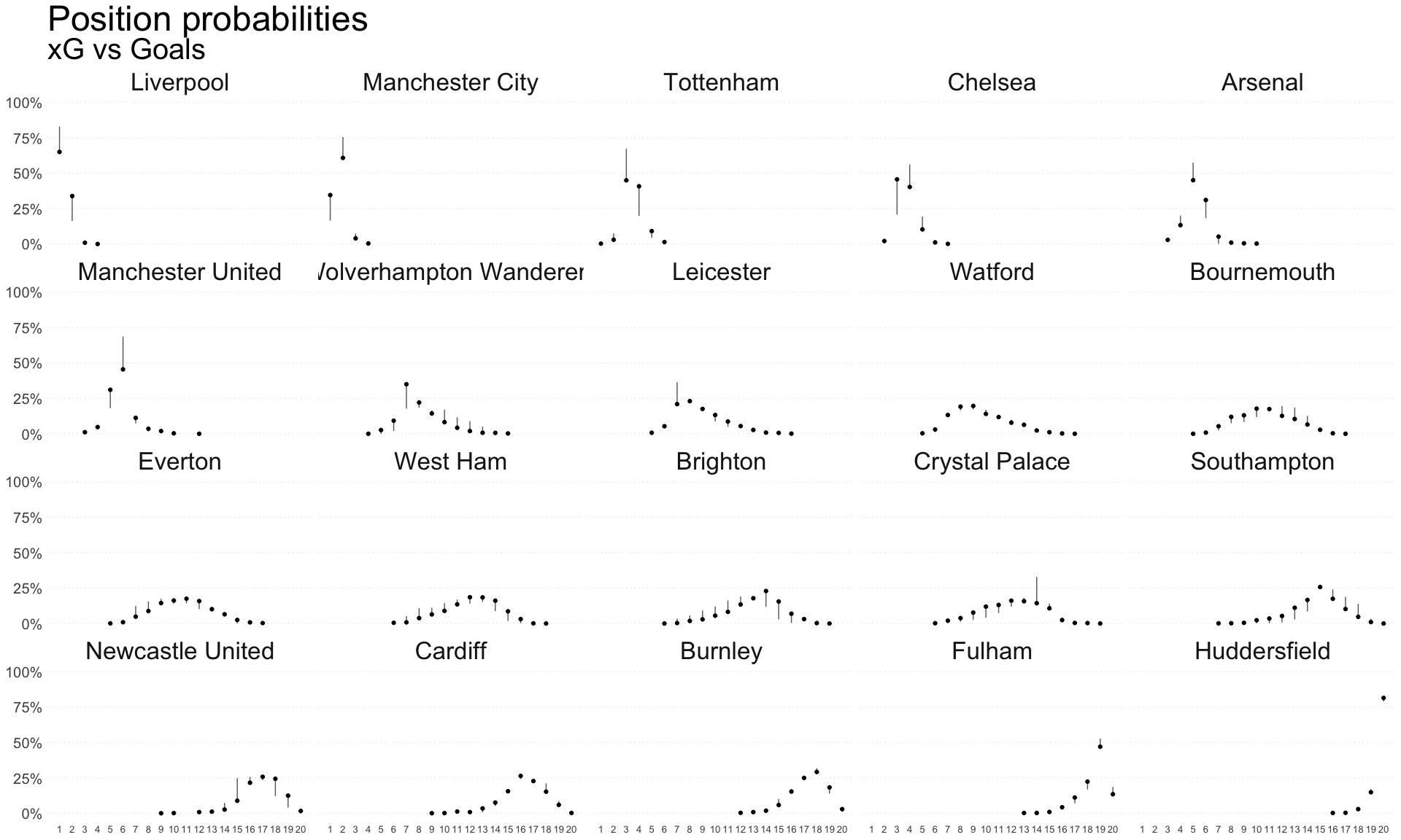
## 1 Liverpool           0.65      0.829
## 2 Manchester City     0.346     0.166

There are fewer big changes in the relegation probablities, but Cardiff and Southampton are probably the biggest winners, while things look more precarious for Burnley and Newcastle:

simulated_tables %>%
group_by(model, team) %>%
summarise(p = mean(position >= 18)) %>%
filter(p > 0.01) %>%
spread(model, p) %>%
arrange(desc(exp_goals))
## # A tibble: 6 x 3
##   team             exp_goals obs_goals
##   <fct>                <dbl>     <dbl>
## 1 Huddersfield         0.993     0.994
## 2 Fulham               0.829     0.882
## 3 Burnley              0.505     0.469
## 4 Newcastle United     0.386     0.164
## 5 Cardiff              0.216     0.308
## 6 Southampton          0.06      0.177

We can look at the race for the Champion’s League, too:

simulated_tables %>%
group_by(model, team) %>%
summarise(p = mean(position <= 4)) %>%
filter(p > 0.01) %>%
spread(model, p) %>%
arrange(desc(exp_goals))
## # A tibble: 6 x 3
##   team              exp_goals obs_goals
##   <fct>                 <dbl>     <dbl>
## 1 Liverpool             1         1
## 2 Manchester City       1         1
## 3 Tottenham             0.893     0.953
## 4 Chelsea               0.882     0.776
## 5 Arsenal               0.164     0.239
## 6 Manchester United     0.06      0.032
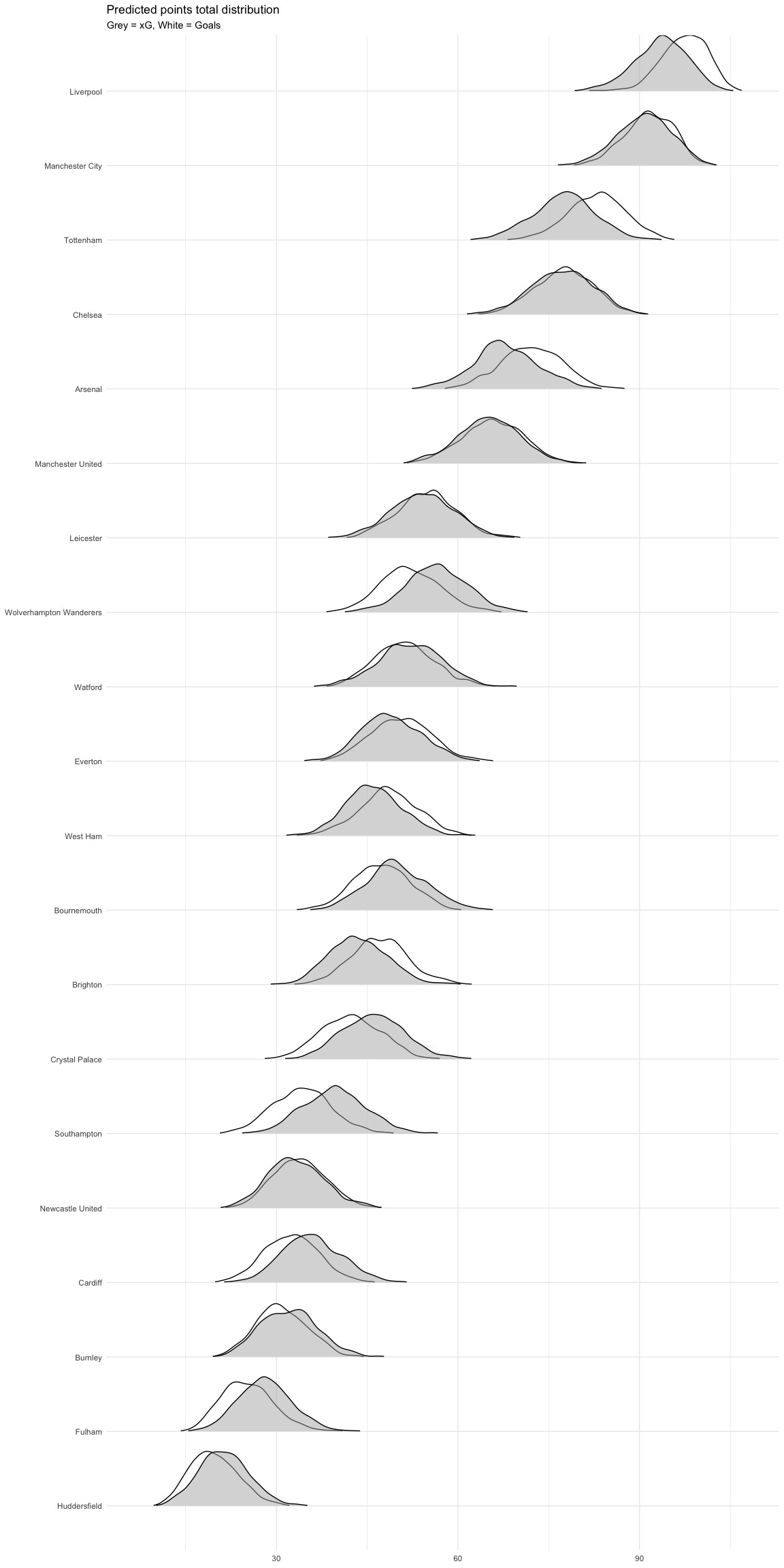
Points totals

We can see how the distribution of points totals changes. The white distribution represents the estimates based on goals, while the grey one refers to those based on xG.

ggplot(data = simulated_tables, aes(x = points, y = reorder(team, points))) +
ggridges::geom_density_ridges(data = simulated_tables %>% filter(model == "obs_goals"),
bandwidth = 1.0,
rel_min_height = 0.01,
scale = 0.75,
fill = "white") +
ggridges::geom_density_ridges(data = simulated_tables %>% filter(model == "exp_goals"),
bandwidth = 1.0,
rel_min_height = 0.01,
scale = 0.75,
alpha = 0.5) +
labs(title = "Predicted points total distribution",
subtitle = "Grey = xG, White = Goals",
x = NULL,
y = NULL) +
theme_minimal()

The xG-based model is less keen on Liverpool’s chances of meeting 100 points. The goal-based model’s dropped its probability by about 10% points since before the Man City game

simulated_tables %>%
group_by(model, team) %>%
summarise(p = mean(points >= 100)) %>%
filter(p > 0.01) %>%
spread(model, p) %>%
arrange(desc(exp_goals))
## # A tibble: 1 x 3
##   team      exp_goals obs_goals
##   <fct>         <dbl>     <dbl>
## 1 Liverpool     0.077      0.31