Does xG really tell us everything about team performance?

Following Liverpool’s decisive title win the end of 2019/20, there was discussion that they might have found a way to “beat” the xG models. The xG tallies suggested that Man City were as good, if not better than Liverpool, but they were left in the dust in the real league table.

Some speculated that it was just random variation, and that Liverpool couldn’t be expected to maintain the over-performance. Others suggested tht their attacking patterns meant that they could create chances better than xG could capture.

This raises the question - how much does xG really tell us? Does it really tell us everything we need to know?

Formulating the question

Let’s start by looking at the two positions at either end of the spectrum:

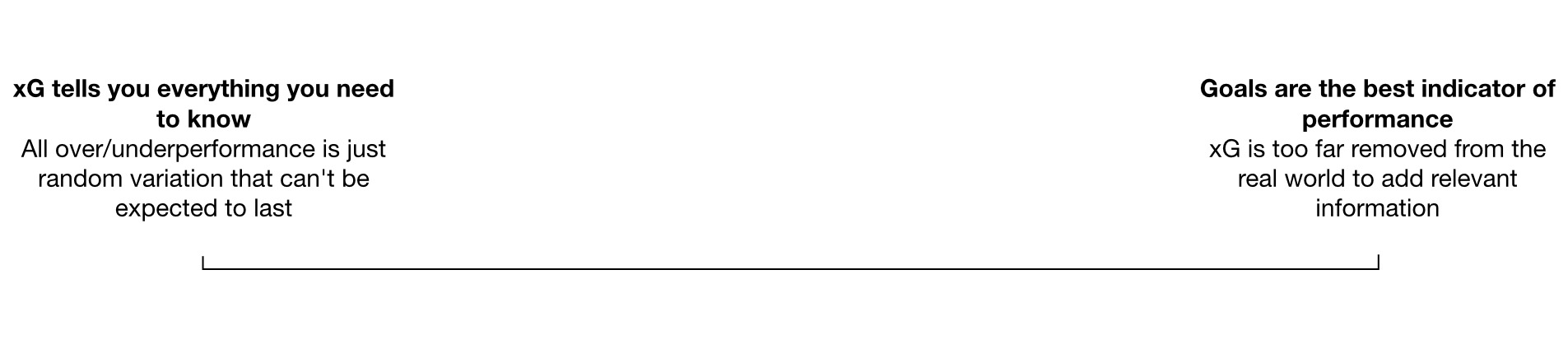
If we had to choose one these two extremes, we already know that only-xG outperforms only-Goals. For a previous post, I created two team-strength models, one using xG data, the other using goals data. I then evaluated the models based on how well each one made predictions about future matches; the xG-based model came out on top.

But there’s a whole lot of space in between the extremes. As Ted Knutson said on Liverpool, “Part of [Liverpool’s 2018-2020 overperformance vs xG] is a little bit of luck. But I think there’s stuff Liverpool do that’s not in the expected goals model”.

So where does the truth lie? If it’s somewhere between the extremes, can we be more specific? And can we prove it?

Ensembles and composing models

The key for us is a technique called ensemble modelling. Ensemble modelling is a technique whereby multiple different models are used to create a single prediction. The intuition is similar to that of wisdom-of-the-crowd; as long as each model is bringing new information that the other model(s) don’t have, then they can improve the prediction accuracy. Thus, a diverse collection of models can perform better than any of the individual constituent models.

To answer our question, we can flip this logic around. We can create a bunch of models across the spectrum of xG-Goals:

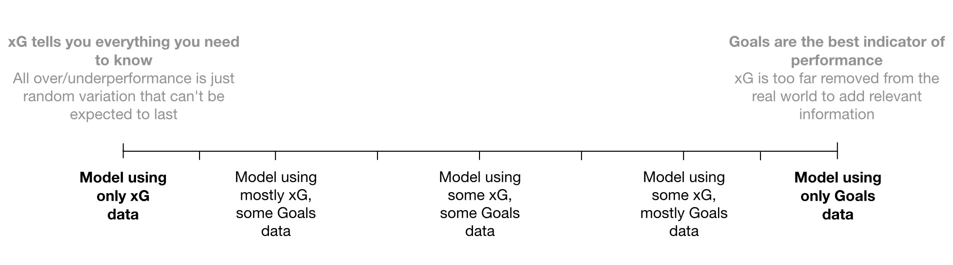
Then, if there’s a combined xG+Goals model that performs better than either xG-only, then goalscoring must be adding information on top of what we already get from xG.

If we plot the model performance for each of these models, we should see one of two shapes^[1], depending on which hypothesis is correct:

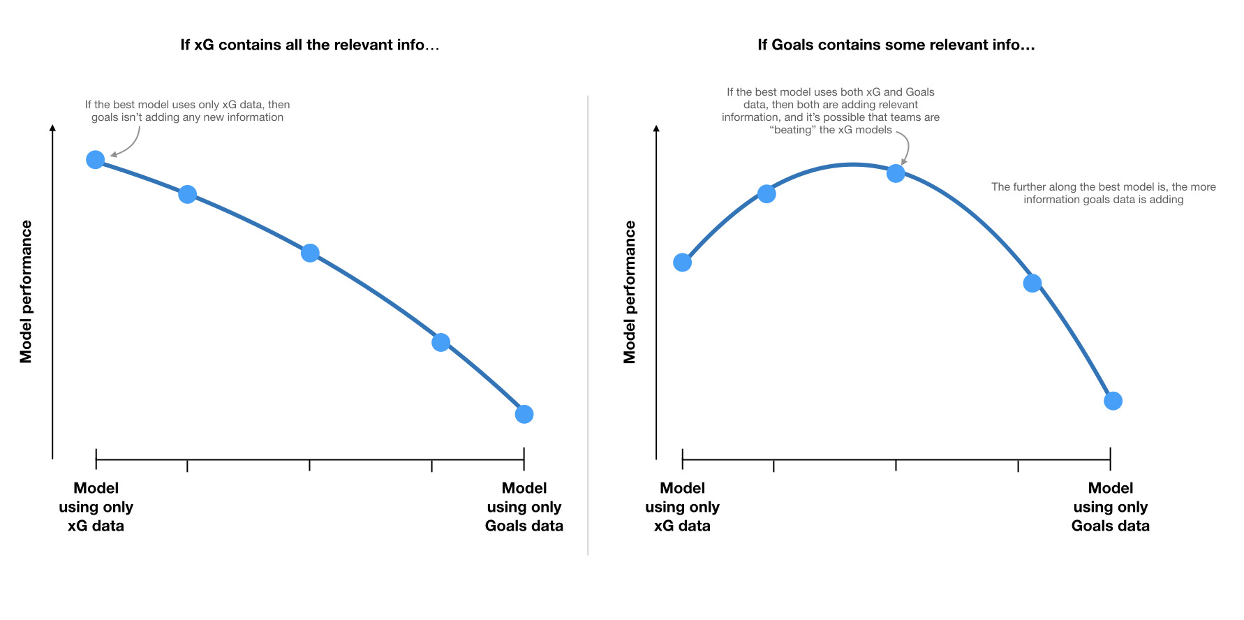
In other words, the location of the best model will tell us where along the spectrum the “truth” lies. If the peak is somewhere in the middle, it would suggest that top performing teams like Liverpool do find some way to outperform the xG models.

How to ensemble team-strength models: technical notes (click to expand)

You might still be wondering how exactly the two models are combined. This requires a little bit of knowledge of how Poisson-based team-strength models work. I think it’s interesting and worth sharing, but feel free to skip ahead if it’s not your bag.

In short, this class of team-strength models contend that the goals scored in a given match are Poisson distributed according to a given rate. (Well, two rates - a home rate for home goals, and an away rate for away goals.)

This rate is the product of a variety of factors: the attacking team’s offensive ability (), the defending team’s defensive ability (), and home advantage (, used in home rate only):

There’s a few more details, which I’ll skip for now (some of my earlier posts go into this a bit more), but this is the most salient part.

The way I see it, there are a few different ways we could combine match prediction models.

1. Combine predictions - Take the predicted scoreline probabilities and take a weighted average. The relative weighting applied to each prediction determines the position along the xG-Goals spectrum.
2. Combine home/away rates - Similar to (1), but the average is taken on the home and away rates of each model, not the scorelines themselves
3. Combine parameters - Similar to (1) and (2), but instead of averaging the predictions, take the average of the parameter estimates themselves.
4. Boost the weighting of actual results (goals data) in the input data - Instead of combining the fitted models (as in 1, 2, and 3), fit the model on combined input data. See this post for more on how input weighting can be used to train team strength models on xG data.

Each of these approaches has some merit. (1) is extremely flexible and could be used to ensemble any match prediction, regardless of it’s internal machinery (random forest, neural networks, and so on). (2) is slightly less flexible, but could be used to combine any Poisson-like models. (3) is more restrictive, since it requires each of the ensembled models to have the same parameters and merely differ in what the estimates of those parameters are. However, this is the method that gives the most insight, since we can inspect the results on a parameter-level. (4) also has the benefit of insight; we could inspect the individual parameter estimates of the new fitted model.

We’re interested in insight and model interpretation, so I figured (3) and (4) were the best fits for this use-case. Of those two, I chose (3), since aggregating the parameter estimates proved to be significantly quicker than fitting an additional set of models.^[2]

Results

The method to evaluate the different models went as follows:

• For each Premier League matchday from the start of 16/17, fit an xG-based model and a Goals-based model on past data (i.e. not including the matchday in question).
• For each matchday, create the combined models, with varying degrees of mixing across the spectrum between xG-only and Goals-only.
• For each model (including the combined models), predict each match taking place on that matchday

This gives a set of 1,860 match predictions with which to evaluate our models. We can evaluate each model’s predictions to get an overall idea of the model’s quality:

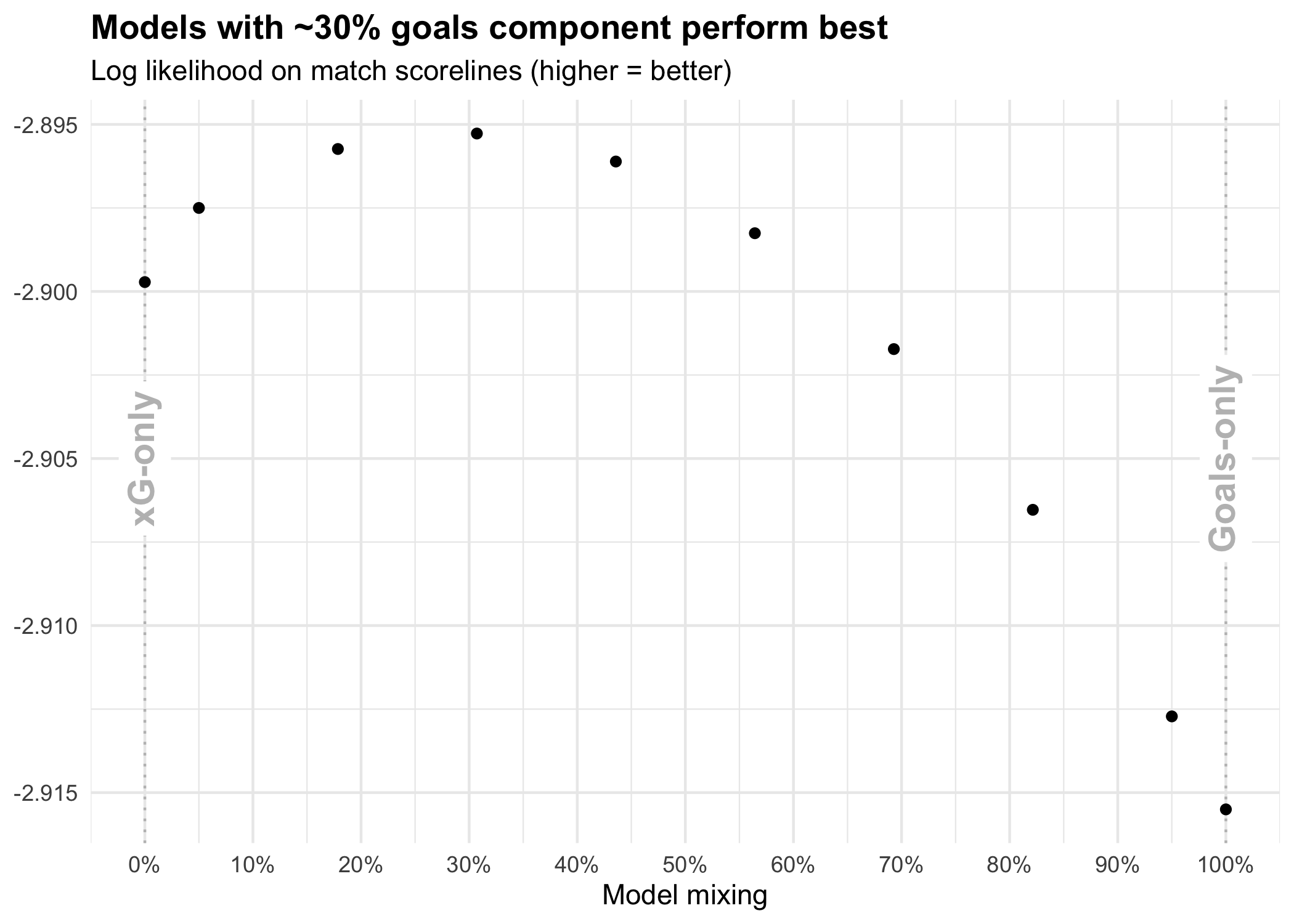
Using log-likelihood as our metric, we get a peak in performance for models with a roughly 30% goals/70% xG component. The exact location of this peak varies depending on how you evaluate the model predictions, but 30% seems like the right approximate figure^[3]. Nonetheless, this suggests that teams with large differences between their xG tallies and actual goals are doing good/bad things that the xG models aren’t picking up on.

The ensemble approach cannot tell us what these unaccounted-for good/bad things are. My hunch is that it’s some combination of:

• Good teams creating more chances with low defensive pressure/clear sight of goal (and vice versa)
• Player finishing skill

Neither of which are included in the xG values used in this analysis.

I used xG data from Understat.com, as that seems to be the defacto public xG model. It’s likely that better xG models, like Statsbomb’s, squeeze the optimal mix of 30% down (more on this later). Although, I think it’s unlikely that it goes all the way to 0%.

What does this look like for individual teams?

Let’s look at the team-strength ratings for the top 6 at the end of 2018/19. This is right in the middle of Liverpool’s red-hot two-year stretch where they recorded the second and fourth-best ever Premier League points tallies.

The team strength ratings are presented in the form of “predicted goals versus an average Premier League team”. In other words, if you played each of these teams against a (hypothetical) perfectly average team over and over again, how many goals would they score and concede on average.

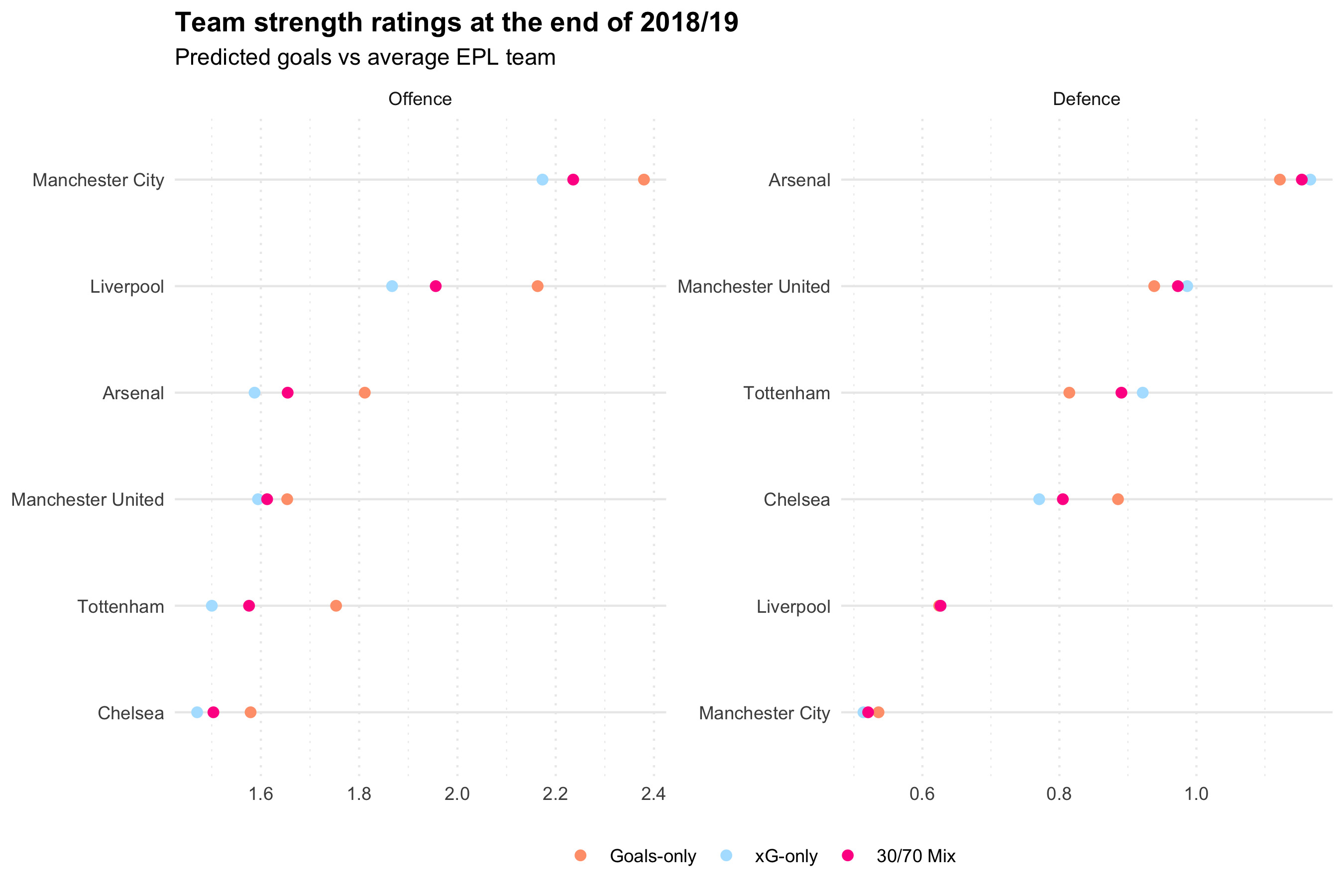
We can see that every one of the top 6 teams was out-performing their xG in attack this season; the goals-only estimate for goals scored (“Offence”) vs average is higher in every case. I think it’s unreasonable to suggest this is just random variation or “luck”. We’re seeing that there’s something missing from the xG values used in this investigation. This suggests that a better xG model (perhaps one built on more detailed data) that helps close the gap between the xG-only and Goals-only models, would have a smaller percentage of Goals-only in the optimal model ensemble.

This doesn’t tell us about whether individual teams are doing things that help them “beat” xG. It doesn’t take into account team tactics, or individual players’ finishing skill. However, it does shift our default expectation of a team’s quality to about 30% of the way between xG and goals.^[4]

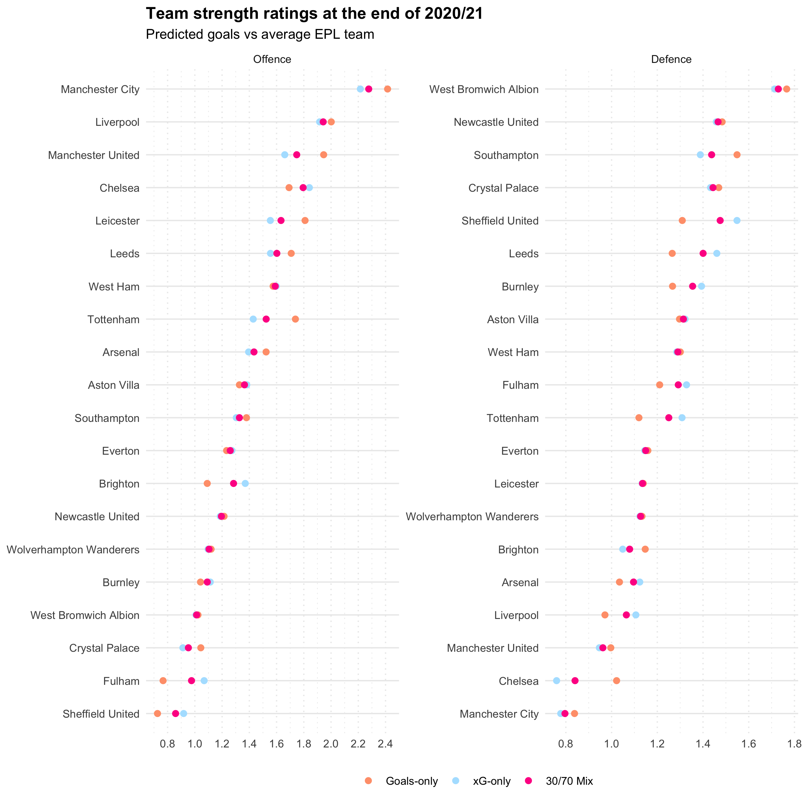
2020/21 ratings

I don’t have anything clever to say, but it’s always fun to look at the most up-to-date ratings:

Conclusions

In general, our best estimate of PL teams’ quality is around 30% between their xG and their Goals, when using xG from Understat.com. Overall this strongly suggests that there is information contained within teams’ goalscoring performance that is not captured by xG totals alone.

On a technical note, this investigation presents a method for combining Poisson-based match prediction models, whilst preserving interpretability of the model parameters. This is useful because the parameter estimates, especially those of team attack and defence ratings, are often of particular interest.

With thanks to Marek Kwiatkowski, Tom Worville and Bobby Gardiner for providing feedback on an earlier draft of this piece.

If you enjoyed this article, I made some Liverpool 2019/20 “data scarves”, which you can buy (if you’re in the UK). I think they’re fun and you might too.

Code etc

If you would like to reproduce this analysis, or dig a bit more into the technical details, the code can be found in my wingback (because it’s concerned with back-testing models… I couldn’t help myself, I’m sorry) repository.

This repo is built on top of understat-db, a project for pulling data from Understat.com into a database. It uses a Python library called mezzala for modelling team-strengths and match predictions.

---

1. I’ve excluded a third scenario where the Goals-only model performs best (a mirror image of xG-only performs best) ↩︎

2. A more patient version of me would have done both (3) and (4) and seen what difference it made (if any). Perhaps something for a future post? ↩︎

3. I looked at log-likelihood on outcomes, mean-squared error (MSE) on per-match total goals and MSE on per-match goal-difference. Each of these gave slightly different results on either side of 30%. ↩︎

4. Since modelled estimates of team quality correlate very closely with total xG/goals scored or conceded, perhaps we could apply this 30/70% rule to xG/Goals totals from Understat, too? ↩︎