Show me the moneyline
Bookmakers’ odds are frequently used as simple predictions for individual games where we don’t care about the underlying model features. While this is useful for running simulations (see this piece on Arsenal), it can also be limiting. Frequently we want estimates of team strength. This information is implicit in the odds (it’s very easy to see which team is better in a given match up, for instance). In this post, I will explore a simple method to extract ratings of team strength from bookmakers’ moneyline (1X2) odds. Having established that team ratings can be easily extracted, these team ratings can be used to create projections for the rest of the season.
To do this, we need to make two slightly dodgy assumptions:
- Bookmakers’ odds can be interpreted as predicted probabilities for a given event occurring.
- We can approximate the model used to get those probabilities.
If you’re not fussed about the method, feel free to skip ahead to the Analysis section at the end.
All the code and methods used in this analysis can be found here.
Unless otherwise stated, all data comes from Joseph Buchdahl’s site football-data.co.uk.
Method
Odds
To convert the odds to probabilities, I will simply be using a linear normalisation. The raw implied odds from bookmakers will add up to more than 1 (the overround). This is to ensure they make a profit. However, we want our probabilities to make sense (i.e. add up to 1). To do this, I divide all the individual probabilities by the overround as per the pseudocode below:
decimal_odds = [1.85, 1.92] # Example (fake) odds |
This method has been shown to be slightly biased. Bookmakers don’t apply the overround to all outcomes evenly. If you want a more accurate estimate, you can use a logistic regression, or one of the other techniques tried by Shin’s model. The size of the bias is tolerable and I’m lazy, so I will continue using linear normalisation for this analysis.
Model
As the title implies, I’m using moneyline (Home/Draw/Away) odds. There are a couple of reasons for doing this. The first is data availability. It is much easier to find historical data for moneyline odds, particularly for closing odds. Finding reliable historical data for handicap and totals odds is hard, even if you’re willing to pay (well, willing to pay a bit).
The second is simplicity. Using handicaps and totals, for instance would require us to split offensive and defensive strength. While this would be more accurate, it also increases the number of assumptions we would have to make. It also increases the sophistication of the analysis and, as I have said earlier, I am lazy.
Instead we will assume an ordinal regression is used to generate the ratings. An ordinal regression is used to create predictions for a set of discrete outcomes that also have a clear order (like match outcomes: home win, draw, away win). There is precedent for these kinds of models in predicting match outcomes. For instance, Koning (2000), used a probit regression to evaluate competitive balance in Dutch soccer. Goddard and Asimakopoulos also used a probit model in their paper Modelling football match results and the efficiency of fixed-odds betting (2003).
I am going to use an ordinal logistic regression as the underlying model.
The maths
In ordinal regression, it is assumed that the probability of an event occuring is a function applied to a linear output. In logistic regression, this function is the logistic function, the inverse of which is the logit function. From here, provided some assumptions about normality and independence (we can check these later), it is simple to coerce the model into a form for linear regression.
Estimating team strengths is then a simple case of running a linear regression where the parameters are the team strengths:
P(event) = logistic(intercept - params*x) |
Results
Next, we want to sense-check the results and check that our assumptions broadly hold. The code used for this analysis is found in full in the R/regression.R file in the github repo. I will be going over this in a bit less detail, so feel free to dig in deeper there.
Our assumptions about normality and independence broadly look okay. The normal Q-Q plot looks a little heavy-tailed. I think we can get away with it for now, but that’s something to bear in mind.
A less academic check we can do is check that the ratings are the same when teams are playing home and away. I did this for each season from 12/13 to 16/17:
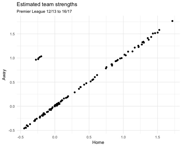
The slope of the line is 0.97, and the intercept is -0.002 (not significantly different to 0). The points at the top left are the different intercepts for home odds and away odds as we expect. There is a trend in both intercepts and it is tempting to suggest that this is home advantage changing over time. This is muddied a bit by how the ratings have been constrained (more on that in a bit) and their lack of interpretability, so I am still unsure if it is just an artefact.
term season away_logit home_logit |
Satisfied that these ratings are basically good enough, we can look at the actual results for each season and sense-check those as well.
As I touched on earlier, the ratings themselves aren’t so interpretable, since they correspond to a wholly unintuitive linear factor used in predicting the log-odds. This isn’t ideal, and we will have to think of them as just abstract relative team strengths.
Another wrinkle comes in the form of adding a constraint. Because ratings are based on differences in team strength there are many valid solutions. For instance, you could shift all ratings by a certain factor and all of the predictions would still be the same, so the model would still be valid.
To fix this, we need to fix a team’s rating to 0 to serve as a baseline. Ideally we want the baseline team to be present in all of our seasons (12/13 to 16/17), without fluctuating much above or below mid-table quality. Obviously, I picked Stoke.
Because of this, ratings aren’t strictly comparable from year to year, as each year’s rating is relative to Stoke’s: 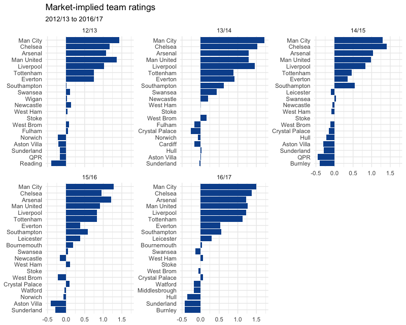
Analysis
Now we have stolen the bookies’ team ratings, there are a few different things we can do.
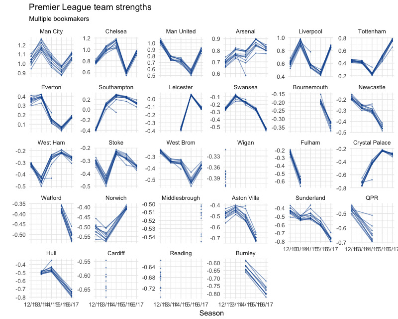
I have rewritten the model in Stan to be a bit more flexible. I have also changed the constraint so that the average rating in each season is 0, so as to be a bit easier to intuit (this was harder to do in the R regression).
Compare bookmakers’ ratings
(see R/plot_strengths.R)
We can see generally close alignment between bookmakers ratings in each season, especially in the trends.
There are quite a few outliers in 2014/15. It turns out that this was Stan James in every case making moves away from the field.
Another thing that stands out is Interwetten being consistently lower on Southampton than the rest of the bookmakers.
Forecast ratings
A more fun thing we can do is use these ratings to simulate the rest of the season. The simulation code is found in project_season.py and the plotting code in R/plot_projection.R.
I simulated the rest of the season 10,000 times using team ratings from Pinnacle’s closing 1X2 odds. This gives the following distribution of points for each team: 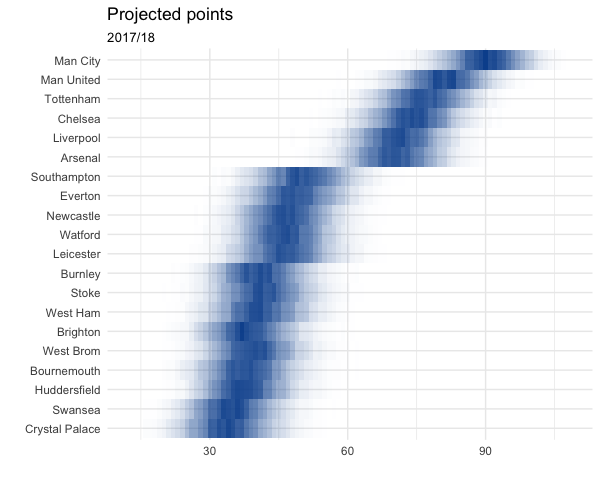
And for finishing position: 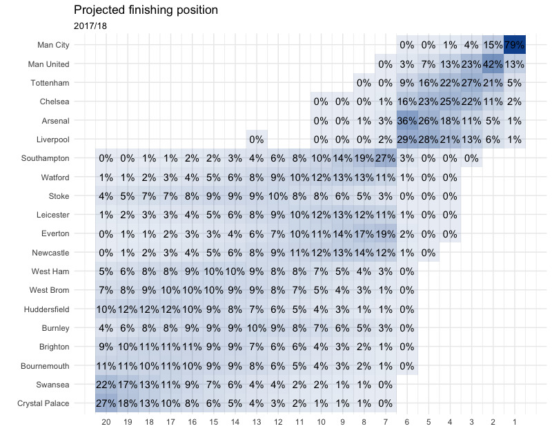
Man City are kinda throwing off the colour scheme a bit…
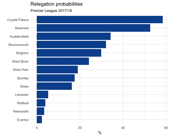
Let’s look at top 4 and relegation probability as well: 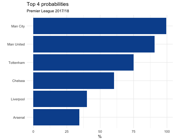
We can also compare to Bookmakers’ outright odds:
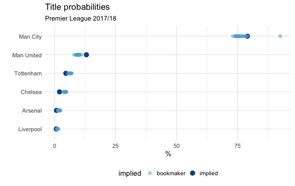
Note that although it looks like Man City are being underrated by the market odds, this effect disappears if you don’t normalise the odds, so don’t go betting on them just yet: 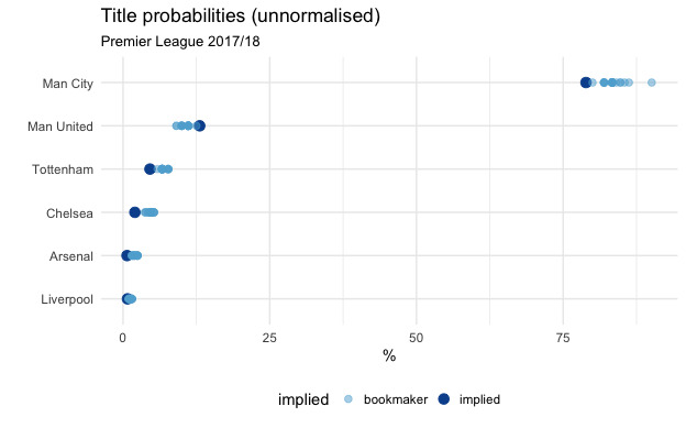
Interestingly, Manchester United’s strength on a game-by-game basis seems to imply that their title chances should be slightly higher than the odds given by the bookies.
It’s tempting to suggest the discrepancies are down to inefficiencies in the betting market. However, the simulation only uses current team strength estimates. It doesn’t account for the myriad possible events that add uncertainty like managerial changes, injuries to key players and the rest.