Are bad shots actually good?
Last month, I saw an interesting tweet from Kees van Hemmen (emphasis is my own):
Correct me if I’m wrong here but, if you’re a low quality side in a league, you’d actually prefer a dozen long shots (lets say each of 0.05 xG) to one great chance (0.6 xG) because there would be a higher variability of outcomes, which would mean you’d have a higher expected points from a given match.
That teams should prioritise high-quality shots has been a common refrain in the public analytics sphere for years. The fact that fewer, high-quality shots can increase win % is even the default example in Danny Page’s Match Expected Goals Simulator.
Over time, there’s been an increasing number of counter-arguments that poor-quality shots (long-shots especially) may have some utility. For example, by keeping a team’s attack from being too predictable, or being a generally positive expected-value way to dispose of a possession.
However, Kees’s hypothesis is particularly interesting because he’s saying that, under certain circumstances (a very bad defence), teams should prefer lots of poor-quality shots, for the same reason that analysts were arguing for high-quality shots: it gets you more points.
What’s the intuition behind this idea?
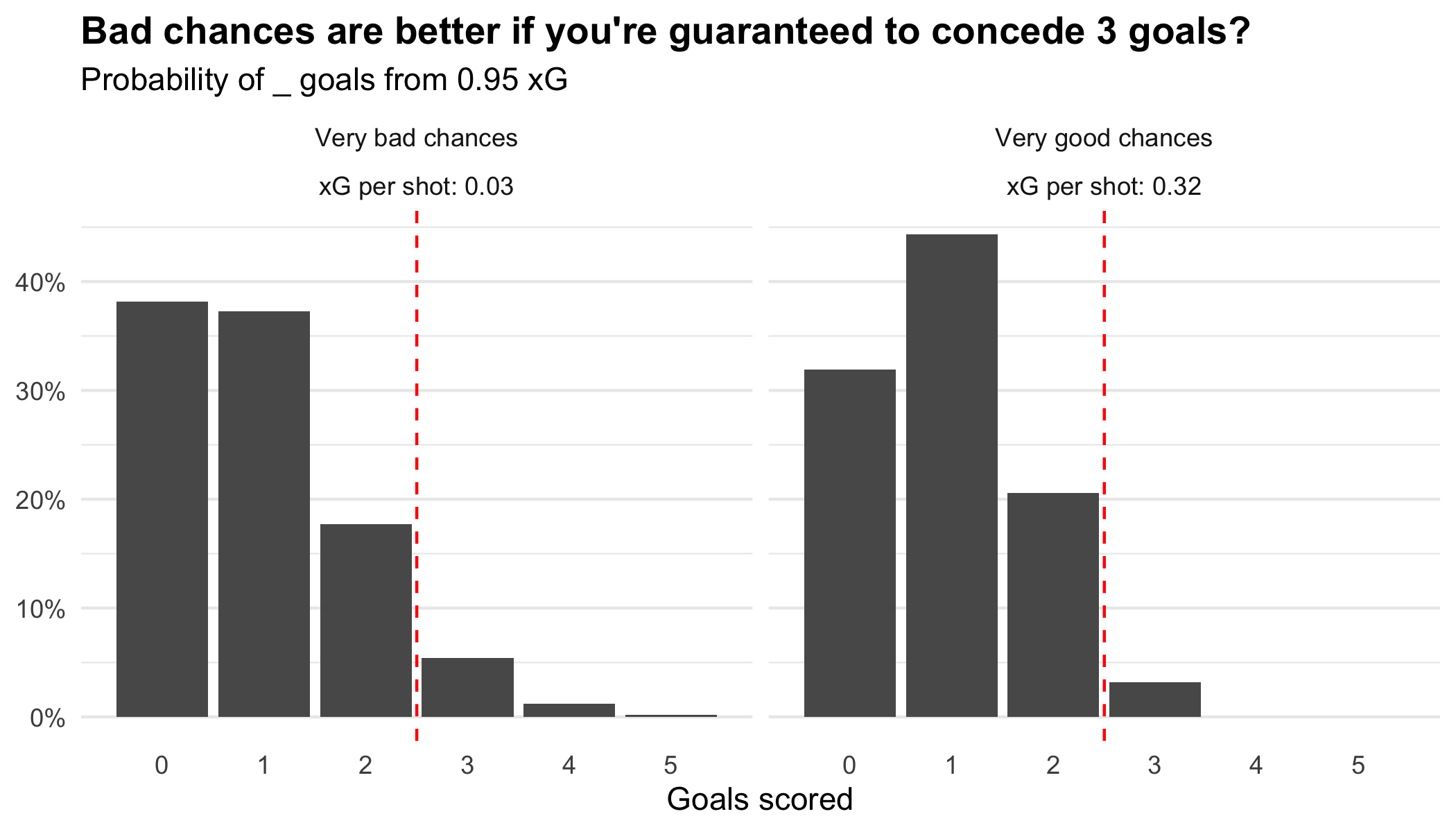
Let’s say we have two teams, who both create 0.95 xG. One of those teams takes 32 shots at about 0.03 xG each (i.e. a 3% chance of scoring each shot). The second team takes just 3 shots (0.32 xG each, 32% chance of scoring each shot). How many goals is each team expected to score?
Expand for R code
library(tidyverse) |
The very bad shots have a greater chance of scoring no goals, and a lower chance of scoring 1 or 2 goals than the very good shots. However, they also have a greater chance of scoring 3 or more goals.
In matches where they concede 2 goals, the first team has a better chance of winning than the second team, despite being less likely to draw. And in matches where 3 goals are conceded, the second team would never do better than a draw! At the bottom end of the table, those extra points can be vital.
So, we can see that there are extreme scenarios where this argument does hold water.
At this point, I should point out that this scenario is adapted from a point that Kees himself made in a follow-up to the original tweet:
One 0.6 xG shot can yield at most one goal, whereas 12 0.05 xG shots can yield many goals but also are more likely to yield none.
But this isn’t an entirely realistic scenario, is it?
In real life, even bad teams keep clean sheets occasionally. This is because the number of goals conceded in a given match follows a distribution. No team consistently concedes 3 goals per game, and even very bad teams keep clean sheets occasionally.
Can we test in a more realistic setting?
I think so! My idea for investigating these dynamics further looks like this:
Take 5 chance quality scenarios, where the total xG generated is a constant 0.95 per game:
Chance quality xG per shot Very bad chances 0.03 Bad chances 0.05 Okay chances 0.10 Good chances 0.19 Very good chances 0.32 And 5 defence quality scenarios, assuming goals conceded per game follow a Poisson distribution:
Defence quality Avg. goals conceded Very bad defence 2.50 Bad defence 1.80 Okay defence 1.30 Good defence 0.90 Very good defence 0.70 Then, see how teams’ chances of getting a result vary for each combination of defence/chance quality, by simulating the goals scored and conceded.
This is, of course, a gross simplification of what the real world looks like. In particular:
- Goals conceded over a season doesn’t actually follow a Poisson distribution. This is driven by variation in the goalscoring rate from match-to-match and within matches.
- We have assumed that goalscoring and goal concession occur independently. In real life, teams’ tactics and motivation is influenced by the scorline.
However, I think this rough approximation is good enough to improve our understanding of the trade-off between attacking chance-quality and results. A more sophisticated model of shot generation developed by Marek Kwiatkowski can be found here, and could form the basis of a more thorough analysis of these trade-offs.
Results
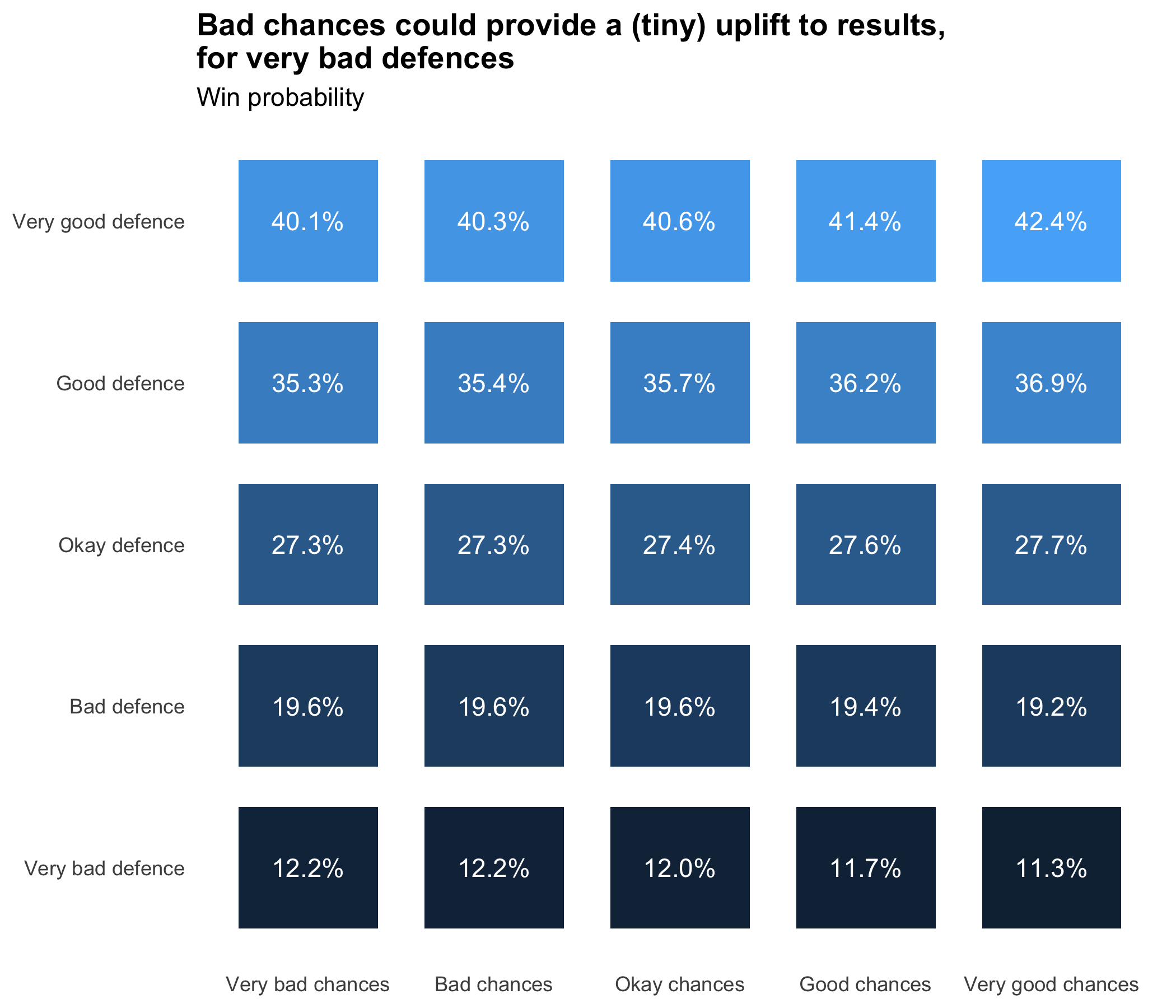
With these assumptions, we can see a very slight uplift to win chance for teams creating 0.95 xG across lower quality chances, when their defence is expected to concede more than about 1.8 goals:
Expand for R code
# NB: continues from previous code section |
However, the uplift to win and draw chance is very small; it is only worth about 0.02 additional expected points. If you’re conceding 3 goals a game, you’re still getting relegated no matter how many long-shots you take.
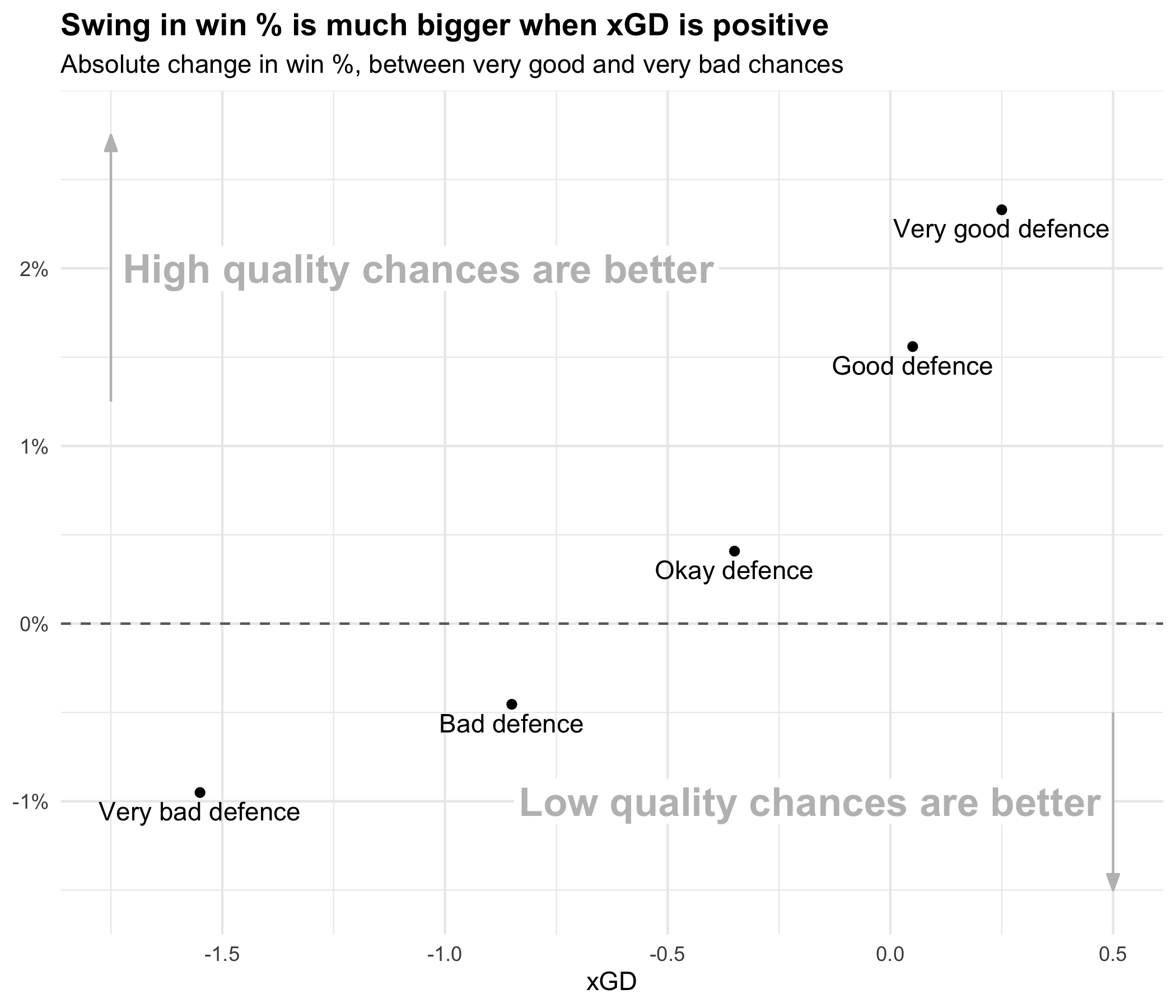
And, as initially noted, there is an advantage gained from having fewer, high-quality chances when generating more xG than your opponent.
This advantage appears to be much more pronounced than the inverse effect (where low-quality chances have the advantage). Teams who are better than their opponents get much more of an uplift from high-quality chances than bad teams get from increasing their variance with low-quality chances.
Expand for R code
annotate_background_text <- partial( |
How should this affect teams decisions?
I don’t think this effect should be a major factor in weak teams’ tactics. The theoretical advantage to weak teams taking low-quality, high-variance shots is very small (maxes out at around 1%). The assumptions made in the above test are rough enough that I don’t think we can sure that such a small edge would even translate into real life.
Moreover, in real matches, you don’t get to distribute the xG of your chances like a character-creation slider in a video game. The strongest case for favouring high-quality chances has always been that, in many cases, playing the right pass will result in a better chance than taking an early shot (even accounting for the fact that the move may break down before a shot can be taken). Does anything we’ve learned here suggest we should move away from a heuristic of “maximise the total xG of each possession sequence”?
For all but the most dominant teams, I would say that it does not.
In matches where a team is dominant, there may be a slight, real advantage gained by prioritising high-quality chances, even at a slight cost to total xG. The method above returns an approximate increase around 4-5% for dominant teams (+1.5 xGD) prioritising very good chances (~0.3 xG per shot), so I think there’s a slightly stronger case to tweak your approach in these circumstances, especially in matches where you’re going to spend a lot of time facing an organised defence.