Estimating the disruption to home advantage

How much has home-field advantage (HFA) been affected by the closed-doors games post-restart?

There have been a few good articles looking at how HFA has been affected in different competitions since returning without crowds. For example, this article in the Economist showing some analysis by 21st Club. The article shows some charts showing the % of total league points won by home teams before and after the restart. These charts are repeated for shots, fouls and some other metrics, with the conclusion:

[T]he lack of help from referees has merely reduced home sides’ advantage, rather than eliminating it… With crowds watching, home teams gained 58% of points; without them, hosts have still earned 56%. In other words, three-quarters of home overperformance remains intact.

In this post, I want to show how to perform a similar analysis using a Dixon-Coles model and the regista R package.

The core of a Dixon-Coles model looks like this:

where

You can read more about it in these posts.

We can make a simple adjustment to this model to capture the HFA before and after the seasons’ interruption: using two separate home advantage parameters. One for pre-interruption, and another for post-interruption.

This requires adjusting the above model to something like

whereis the home advantage parameter for pre-interruption games. For post-restart games, this parameter is fixed to 1, and thus has no effect. The inverse is true for.

Loading the data

First off, we need some data from before and after the COVID-enforced break. I am using data for the 2019/20 season in the Premier League, Serie A, Bundesliga, and La Liga.

In this post, I’m using a modified approach to the standard Dixon-Coles model that allows the use of xG as an input to team strengths. To do this, we need to load in xG value of each shot in any relevant matches.

The data used in this post comes from Understat. Since obtaining this data is not the core message of this post, I have left the code for this part out. However, you can find the R code used to scrape the data at the this link.

If you have access to a broader dataset, or data from a different provider, I encourage you to experiment with re-running the analysis on that data. The only code chunk you should need to edit is the following one. The rest of the chunks should be plug and play, provided the column names of the shots dataframe remain the same as the ones below.

library(tidyverse)

shots <-
  # EDIT HERE
  # Each row of this CSV refers to a single shot
  read_csv(here::here("data", "understat-shots.csv")) %>%
  # If using your own data source, select and rename your own column names
  # below for the rest of the analysis to run
  transmute(
    match_id,
    league_name,
    match_date = lubridate::as_date(datetime),
    is_home    = h_a == "h" ,
    home_team  = h_team,
    away_team  = a_team,
    home_goals = h_goals,
    away_goals = a_goals,
    xG
  )

# Preview the data
sample_n(shots, 10)

## # A tibble: 10 x 9
##    match_id league_name match_date is_home home_team           away_team      home_goals away_goals     xG
##       <dbl> <chr>       <date>     <lgl>   <chr>               <chr>               <dbl>      <dbl>  <dbl>
##  1    12702 Bundesliga  2020-06-27 TRUE    Borussia M.Gladbach Hertha Berlin           2          1 0.110
##  2    13246 Serie A     2019-12-15 FALSE   AC Milan            Sassuolo                0          0 0.0128
##  3    13194 Serie A     2019-11-03 TRUE    Lecce               Sassuolo                2          2 0.108
##  4    12336 La liga     2020-06-28 FALSE   Espanyol            Real Madrid             0          1 0.469
##  5    13252 Serie A     2020-02-05 TRUE    Lazio               Verona                  0          0 0.0684
##  6    12705 Bundesliga  2020-06-27 FALSE   Werder Bremen       FC Cologne              6          1 0.422
##  7    11818 EPL         2019-12-21 FALSE   Newcastle United    Crystal Palace          1          0 0.0456
##  8    11842 EPL         2019-12-28 FALSE   West Ham            Leicester               1          2 0.761
##  9    11838 EPL         2019-12-28 FALSE   Newcastle United    Everton                 1          2 0.528
## 10    13344 Serie A     2020-02-29 TRUE    Napoli              Torino                  2          1 0.0753

Preparing the data

The next step is to split the shots taken by the home and away team into separate groups:

match_xgs <-
  shots %>%
  group_by(match_id, league_name, match_date, home_team, away_team, home_goals, away_goals) %>%
  summarise(home_xgs = list(discard(ifelse(is_home, xG, NA), is.na)),
            away_xgs = list(discard(ifelse(!is_home, xG, NA), is.na))) %>%
  ungroup()

match_xgs

## # A tibble: 1,407 x 9
##    match_id league_name match_date home_team         away_team               home_goals away_goals home_xgs   away_xgs
##       <dbl> <chr>       <date>     <chr>             <chr>                        <dbl>      <dbl> <list>     <list>
##  1    11643 EPL         2019-08-09 Liverpool         Norwich                          4          1 <dbl [15]> <dbl [13]>
##  2    11644 EPL         2019-08-10 West Ham          Manchester City                  0          5 <dbl [5]>  <dbl [14]>
##  3    11645 EPL         2019-08-10 Bournemouth       Sheffield United                 1          1 <dbl [13]> <dbl [8]>
##  4    11646 EPL         2019-08-10 Burnley           Southampton                      3          0 <dbl [10]> <dbl [11]>
##  5    11647 EPL         2019-08-10 Crystal Palace    Everton                          0          0 <dbl [6]>  <dbl [10]>
##  6    11648 EPL         2019-08-10 Watford           Brighton                         0          3 <dbl [12]> <dbl [5]>
##  7    11649 EPL         2019-08-10 Tottenham         Aston Villa                      3          1 <dbl [31]> <dbl [7]>
##  8    11650 EPL         2019-08-11 Newcastle United  Arsenal                          0          1 <dbl [9]>  <dbl [8]>
##  9    11651 EPL         2019-08-11 Leicester         Wolverhampton Wanderers          0          0 <dbl [16]> <dbl [8]>
## 10    11652 EPL         2019-08-11 Manchester United Chelsea                          4          0 <dbl [11]> <dbl [18]>
## # … with 1,397 more rows

From here, we can generate the features for an “xG-Dixon-Coles” model. This involves “re-simulating” each match based on the shots taken within it, to get a set of weighted scorelines. For more on this method, see this post.

We also generate two new variables corresponding to the two home advantage parameters: pre_restart and post_restart.

simulate_shots <- function(xgs) {
  tibble::tibble(goal = 0:length(xgs),
                 prob = poisbinom::dpoisbinom(0:length(xgs), xgs))
}

simulate_game <- function(home_xgs, away_xgs) {
  home_probs <- simulate_shots(home_xgs) %>% dplyr::rename_all(function(x) paste0("h", x))
  away_probs <- simulate_shots(away_xgs) %>% dplyr::rename_all(function(x) paste0("a", x))

  tidyr::crossing(home_probs, away_probs) %>%
    dplyr::mutate(prob = .data$hprob * .data$aprob)
}


simulated_games <-
  match_xgs %>%
  mutate(simulated_probabilities = map2(home_xgs, away_xgs, simulate_game),
         pre_restart  = match_date < "2020-05-01",
         post_restart = !pre_restart) %>%
  unnest(cols = c(simulated_probabilities)) %>%
  filter(prob > 0.01)

simulated_games

## # A tibble: 20,694 x 16
##    match_id league_name match_date home_team away_team home_goals away_goals home_xgs away_xgs hgoal  hprob agoal  aprob
##       <dbl> <chr>       <date>     <chr>     <chr>          <dbl>      <dbl> <list>   <list>   <int>  <dbl> <int>  <dbl>
##  1    11643 EPL         2019-08-09 Liverpool Norwich            4          1 <dbl [1… <dbl [1…     0 0.0556     0 0.398
##  2    11643 EPL         2019-08-09 Liverpool Norwich            4          1 <dbl [1… <dbl [1…     0 0.0556     1 0.405
##  3    11643 EPL         2019-08-09 Liverpool Norwich            4          1 <dbl [1… <dbl [1…     1 0.230      0 0.398
##  4    11643 EPL         2019-08-09 Liverpool Norwich            4          1 <dbl [1… <dbl [1…     1 0.230      1 0.405
##  5    11643 EPL         2019-08-09 Liverpool Norwich            4          1 <dbl [1… <dbl [1…     1 0.230      2 0.158
##  6    11643 EPL         2019-08-09 Liverpool Norwich            4          1 <dbl [1… <dbl [1…     2 0.328      0 0.398
##  7    11643 EPL         2019-08-09 Liverpool Norwich            4          1 <dbl [1… <dbl [1…     2 0.328      1 0.405
##  8    11643 EPL         2019-08-09 Liverpool Norwich            4          1 <dbl [1… <dbl [1…     2 0.328      2 0.158
##  9    11643 EPL         2019-08-09 Liverpool Norwich            4          1 <dbl [1… <dbl [1…     2 0.328      3 0.0337
## 10    11643 EPL         2019-08-09 Liverpool Norwich            4          1 <dbl [1… <dbl [1…     3 0.241      0 0.398
## # … with 20,684 more rows, and 3 more variables: prob <dbl>, pre_restart <lgl>, post_restart <lgl>

Estimating the home advantage

For each league, we are going to fit the aforementioned model with two separate home advantage parameters.

Because we are extending the core Dixon-Coles model, we must use the more flexible dixoncoles_ext function. This function allows us to specify custom formulas for the home (f1) and away (f2) goals estimates with extra parameters, such as our pre_/post_restart HFA parameters.

library(regista)

fit_model <- partial(
  dixoncoles_ext,
  f1 = hgoal ~ off(home_team) + def(away_team) + pre_restart + post_restart + 0,
  f2 = agoal ~ off(away_team) + def(home_team) + 0,
  weights = prob
)


models <-
  simulated_games %>%
  group_by(league_name) %>%
  nest() %>%
  mutate(model = map(data, fit_model)) %>%
  ungroup()

models

## # A tibble: 4 x 3
##   league_name data                  model
##   <chr>       <list>                <list>
## 1 EPL         <tibble [5,456 × 15]> <dixoncls>
## 2 La liga     <tibble [5,110 × 15]> <dixoncls>
## 3 Bundesliga  <tibble [4,804 × 15]> <dixoncls>
## 4 Serie A     <tibble [5,324 × 15]> <dixoncls>

We can extract the parameter estimates from the models with broom::tidy. While the model will estimate attack and defence strengths for each team too, we specifically care about the estimates for pre_restart and post_restart.

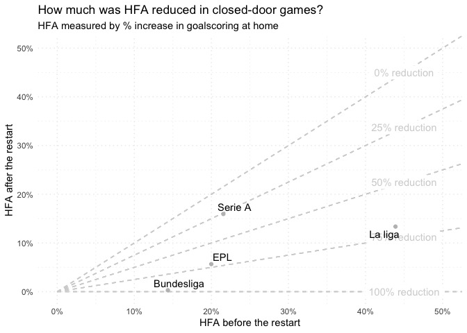
So, let’s take these and compare the before and after estimates:

model_parameters <-
  models %>%
  mutate(params = map(model, broom::tidy)) %>%
  select(league_name, params) %>%
  unnest(params)

hfa_comparison <-
  model_parameters %>%
  mutate(value = exp(value)) %>%  # Get the value out of log space...
  filter(str_detect(parameter, "(pre|post)_restart")) %>%
  pivot_wider(id_cols = league_name, names_from = parameter, values_from = value)


hfa_comparison %>%
  ggplot(aes(x = pre_restart - 1, y = post_restart - 1)) +

  map(seq(0, 1, by = 0.25), function(slope) {
    list(
      geom_segment(x = 0, y = 0, xend = 1.5, yend = slope*1.5, linetype = "dashed", colour = "lightgray"),
      annotate(geom = "label", x = 0.45, y = slope*0.45,
               label = str_glue("{scales::percent(1 - slope, 1)} reduction"),
               colour = "lightgray", label.size = 0)
    )
  }) +

  ggrepel::geom_text_repel(aes(label = league_name)) +
  geom_point(aes(colour = (post_restart / pre_restart) < 0.97)) +
  scale_x_continuous(limits = c(0, 0.5), labels = scales::percent_format(accuracy = 1)) +
  scale_y_continuous(limits = c(0, 0.5), labels = scales::percent_format(accuracy = 1)) +
  scale_colour_manual(values = c("gray", "red"), guide = FALSE) +
  theme_minimal() +
  theme(panel.grid.major = element_line(linetype = "dotted"),
        panel.grid.minor = element_line(linetype = "dotted")) +
  labs(title = "How much was HFA reduced in closed-door games?",
       subtitle = "HFA measured by % increase in goalscoring at home",
       x = "HFA before the restart",
       y = "HFA after the restart")